

An illustration to create ML class for different hyper-parameter tuning techniques
This article is for the new and aspirant data scientists to demonstrate the use of object oriented programming in Python to tune the machine learning (ML) models . So, if you’re new and growing in love with this amazing field you would have realized certain milestones in your learning curve, first you would be brushing your statistics skills and then learn about visualization and data transformation with tools like numpy and pandas and then finally would create and test your machine learning models. The next progression is to familiarize yourself with object-oriented programming (OOP) and starting to write the Python scripts. By, the end of this article you would have some understanding parameter tuning and creating the class object for ML models. The article is divided into 2 parts so suit yourself to jump to the section you feel is appropriate for you (checkout the notebook).
- Introduction to Bayesian Optimization
- ML Object Classes for hyper-parameter tuning
Introduction to Bayesian Optimization
Not too long ago selection of hyper-parameters was termed as the ‘art’, some would say it requires skills to tune while others would say it’s based on intuition. Additionally, the more complex the ML algorithm gets the more are the hyper-parameters to tune. In such scenarios one option is to tune the model with every possible tuning combination aka grid search also known as brute force. Or another approach is to test the hyper-parameters with trial and error and picking parameter sets at random. The latter approach is preferred than the former as there is better chance of identifying the well performing parameters. Both random search and grid search are available in sklearn library with cross validation.
Fortunately, there are better ways to tune the hyper-parameters which are more effective than a random search like Bayesian Optimization, which arrives on the best hyper-parameter values by estimating and updating the probability distribution that describes potential values of the objective function. In simple word this means when the algorithm finds a good result for particular value of a hyper-parameter it intensifies the search around that value. We would discuss two python libraries Hyperopt and Optuna which use such approach.
Hyperopt has excellent tutorial, we would demonstrate its use on a LightGBM model. The gradient boosted tree algorithms are very popular for building supervised learning models and LightGBM is a great type in it. We would use breast cancer dataset in sklearn
\# importing the essential libraries
import numpy as np
import pandas as pd
import lightgbm as lgb
from sklearn.model\_selection import train\_test\_split
from sklearn.metrics import f1\_score, confusion\_matrix, classification\_report\# importing the dataset
from sklearn.datasets import load\_breast\_cancer
\# importing the hyperopt methods
from hyperopt import fmin, hp, tpe, Trials, STATUS\_OKdataset = load\_breast\_cancer()X = dataset.data
y = dataset.targetX\_train, X\_test, y\_train, y\_test = train\_test\_split(X, y, train\_size = 2/3, random\_state = 1)
Four methods have been called from Hypeopt library — fmin, hp, tpe and STATUS_OK. The first, fmin is the method that minimizes the objective function loss. If we want our model to perform with higher accuracy then what we would like to minimize is (1-accuracy) in same way if we want to minimize the F1score, the loss that we would minimize is (1-F1score) as shown below:
#lgb model takes param as dict
param = {'objective': 'binary', 'learning\_rate': 0.5,'reg\_alpha': 0.5, 'reg\_lambda': 0.5}
model = lgb.train(params, lgb.Dataset(X\_train, label = y\_train))
\# lgb mode.predict gives predict probabilities
pred=h\_model.predict(X\_test)
\# defining predicted label based on 0.5 threshold
y\_pred = np.where(pred>0.5,1,0)\# claculating the f1 score
f1sc = f1\_score(y\_test, y\_pred
\>>0.9561752988047808
loss = 1-f1sc
\>>0.0438247011952192
In the codes above, the hyperopt fmin method could be used to optimize the loss i.e. help to improve the F1score. To create such function we would want it to take different hyper-parameters as input and test improvement in F1score. Therefore, we could do the following:
def objective(params):\# an objective function
  h\_model = lgb.train(params, lgb.Dataset(X\_train, label = y\_train))
  pred=h\_model.predict(X\_test)
  y\_pred = np.where(pred>0.5,1,0)
  f1sc = f1\_score(y\_test, y\_pred)
  loss = 1 — f1sc
  return {‘loss’: loss, , 'status' : STATUS\_OK}
This objective function would be optimized on whatever is defined as loss. Next we need a parameter space from where the value of hyper-parameters would be selected. Such search space is defined by hp:
\# quniform: quantile uniform distribution (discrete);
space = {
         ‘lambda\_l1’: hp.uniform(‘lambda\_l1’, 0.0, 1.0),
         ‘lambda\_l2’: hp.uniform(“lambda\_l2”, 0.0, 1.0),
         ‘learning\_rate’ : hp.loguniform(‘learning\_rate’,                                                                                                      np.log(0.05), np.log(0.25)),
         ‘objective’ : ‘binary’}
trials = Trials()
The tpe method has algorithm to search from the space defined above and Trials method creates a database to to record the trials. And finally STATUS_OK which is mandatory to be returned from objective function to store the success of the run. The fmin method would store results - best parameters chosen from hyper-parameter space.
best = fmin(fn=objective, space=space, algo=tpe.suggest, max\_evals=1000)
best
output> {'lambda\_l1': 0.0021950856879321273,  'lambda\_l2': 0.004537789645112988,  'learning\_rate': 0.10215913897624063,  'num\_leaves': 176.0}
Notice that when fmin method is called we also have to specify the number of maximum evaluation or the number of time the space would be searched to predict the optimum parameters.
Optuna library too optimizes the hyper-parameters with Bayesian Optimization. But there is ease in coding over Hyperopt, firstly, we define objective function and hyper-parameter space inside a single function. Secondly, unlike Hyperopt which only ‘minimizes’ the objective function in Optuna we could define if we wish to maximize or minimize the objective.
import optunadef optuna\_obj(trial):
  '''Defining the parameters space inside the function for optuna optimization''' params = {‘num\_leaves’: trial.suggest\_int(‘num\_leaves’, 16, 196, 4),
  ‘lambda\_l1’: trial.suggest\_loguniform(‘lambda\_l1’, 1e-8, 10.0),
  ‘lambda\_l2’: trial.suggest\_loguniform(“lambda\_l2”, 1e-8, 10.0),
  ‘learning\_rate’ : trial.suggest\_loguniform(‘learning\_rate’, 0.05, 0.25)} o\_model = lgb.train(params, lgbo.Dataset(X\_train, label = y\_train))pred=o\_model.predict(X\_test)
  y\_pred = np.where(pred>0.5,1,0)
  f1sc = f1\_score(y\_test, y\_pred)
  loss = 1 — f1sc
  return lossstudy = optuna.create\_study(direction=’minimize’)
study.optimize(optuna\_obj, n\_trials=2000)
Notice that we have used ‘minimize’ as direction since we want an output similar to Hyperopt. We could have also returned f1-score with direction as ‘maximum’ in Optuna. The optimized hyper-parameters are stored in best_params attribute in study.
study.best\_params
\>> {'lambda\_l1': 9.81991399439663e-07,  'lambda\_l2': 4.23211064923651,  'learning\_rate': 0.1646975912311242,  'num\_leaves': 64}
We should observe that our initial parameters and the best parameters from Hyperopt and Optuna are all different. While it is understandable for manually defined parameters to be different, the reason for different Optuna and Hyperopt best parameters could lie with maximum evaluation and the internal algorithm’s approach in optimizing. The f1-score does improve with the new parameters
ML Object Classes for hyper-parameter tuning
The focus in this section would be to demonstrate how to create a classifier class. There are plenty of resources available on OOP programming but demonstration of complete classes is limited. We would use the above example to create a class. In building a class it is important to visualize the structure of your class, here we would create a simple flow as shown in the figure below.
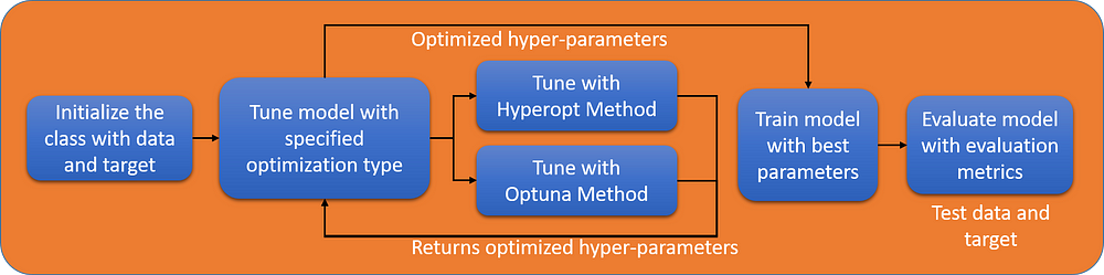
Structure of defined ML class
The overall structure of the above class would be something like:
class Mlclass():
  def \_\_init\_\_(self,...):
    ...
  def tuning(self, ...):
    ...
  def hyperopt\_method(self):
    ...
  def optuna\_method(self):
    ...
  def train(self):
    ...
  def evaluate(self):
    ...
This basic structure would give us a good understanding of different types of class methods, there are some methods like tuning, train and evaluate which would be called by the user while others like hyperopt and optuna would be used within the class without requiring user to call them.
class MLclass():
  '''Parameter Tuning Class tunes the LightGBM model with different   optimization techniques - Hyperopt, Optuna.''' def \_\_init\_\_(self, x\_train, y\_train):
    '''Initializes the Parameter tuning class and also initializes   LightGBM dataset object
    Parameters
    ----------
    x\_train: data (string, numpy array, pandas DataFrame,or list of numpy arrays) – Data source of Dataset. y\_train: label (list, numpy 1-D array, pandas Series / one-column DataFrame or None – Label of the data.''' self.x\_train = x\_train
    self.y\_train = y\_train
    self.train\_set = lgb.Dataset(data=train\_X, label=train\_y)
The ML class method is first initialized with training dataset and the target. A class is defined by starting with class. The functions defined inside the class are known as methods. Our first method is __init__ which is used to initialize the class. Here we want our class to be initialized with data-set and the target so we have given the inputs parameters as ‘x_train’ and ‘y_train’. The self in the method is used to associate the function with an instance. Using ‘self. ‘ as prefix to the variables also makes the class variables specific to that instance. Calling this class is as easy as:
#defining a unique class object
obj = MLclass(X\_train, y\_train)
Once the class method is initialized we would add the method for Hypeorpt optimization. We would want user to input optimization type as Hypeorpt and then tune the model.
def tuning(self, optim\_type):
  '''Method takes the optimization type and tunes the model'''
  #call the optim\_type: Hyperopt or Optuna
  optimization = getattr(self, optim\_type)
  return optimization()def hyperopt\_method(self):
  # This method is called by tuning when user inputs   'hyperopt\_method' while calling the tuning method
  #define the hyperopt space
  space = {'lambda\_l1': hp.uniform('lambda\_l1', 0.0, 1.0),
  'lambda\_l2': hp.uniform("lambda\_l2", 0.0, 1.0),
  'learning\_rate' : hp.loguniform('learning\_rate',
np.log(0.05), np.log(0.25)),
  'objective' : 'binary'} # define algorithm and trials inside the class
  algo, trials= tpe.suggest, Trials() #Call the fmin from inside the class
    best=fmin(fn=objective,space=space,algo=algo,trials=trials,max\_evals=1000)
  self.params = best
  return best, trialsdef objective(self, params):
  # same objective function with added self
  h\_model = lgb.train(params, lgb.Dataset(X\_train, label = y\_train))
  pred=h\_model.predict(X\_test)
  y\_pred = np.array(list(map(lambda x: int(x), pred>0.5)))
  f1sc = f1\_score(y\_test, y\_pred)
  loss = 1 - f1sc
  return {'loss': loss,'status' : STATUS\_OK}#call the tuner method
obj.tuning('hyperopt\_method')return optimization()def hyperopt\_method(self):\# This method is called by tuning when user inputs 'hyperopt\_method' while calling the tuning method#define the hyperopt spacespace = {'lambda\_l1': hp.uniform('lambda\_l1', 0.0, 1.0),'lambda\_l2': hp.uniform("lambda\_l2", 0.0, 1.0),'learning\_rate' : hp.loguniform('learning\_rate',np.log(0.05), np.log(0.25)),'objective' : 'binary'}\# define algorithm and trials inside the classalgo, trials= tpe.suggest, Trials()#Call the fmin from inside the classbest = fmin(fn=objective,space=space,algo=algo,trials=trials,max\_evals=1000)self.params = bestreturn best, trialsdef objective(self, params):\# same objective function with added selfh\_model = lgb.train(params, lgb.Dataset(X\_train, label = y\_train))pred=h\_model.predict(X\_test)y\_pred = np.array(list(map(lambda x: int(x), pred>0.5)))f1sc = f1\_score(y\_test, y\_pred)loss = 1 - f1screturn {'loss': loss,'status' : STATUS\_OK}#call the tuner method
obj.tuning('hyperopt\_method')
When the tuning method is called as in the codes above, Hyperopt optimization would be performed. Let’s define a similar method for Optuna
def optuna\_method(self):
  study = optuna.create\_study(direction=’minimize’)
  study.optimize(optuna\_obj, n\_trials=2000)
  self.params = study.best\_params
  return studydef optuna\_obj(self, trial):
  '''Same optuna objective with parameters space inside the function for optuna optimization''' params = {‘num\_leaves’: trial.suggest\_int(‘num\_leaves’, 16, 196, 4),
  ‘lambda\_l1’: trial.suggest\_loguniform(‘lambda\_l1’, 1e-8, 10.0),
  ‘lambda\_l2’: trial.suggest\_loguniform(“lambda\_l2”, 1e-8, 10.0),
  ‘learning\_rate’ : trial.suggest\_loguniform(‘learning\_rate’, 0.05, 0.25)} o\_model = lgb.train(params, lgbo.Dataset(X\_train, label = y\_train)) pred=o\_model.predict(X\_test)
  y\_pred = np.array(list(map(lambda x: int(x), pred>0.5)))
  f1sc = f1\_score(y\_test, y\_pred)
  loss = 1 — f1sc
  return loss#calling tuner with optuna
obj.tuning('optuna\_method')
To use the best parameters for evaluation we defined another variable self.params which would be defined for that instance and could be accessed by a yet to be defined train method.
def train(self):
  """This function evaluates the model on best parameters"""
print("Model will be trained on the following parameters: \\n{}".format(self.params)) #train the model with best parameters
  self.gbm = lgb.train(self.params, self.train\_set)obj.train()
\>> Model will be trained on the following parameters:
\>>{'lambda\_l1': 9.81991399439663e-07,  'lambda\_l2': 4.23211064923651,  'learning\_rate': 0.1646975912311242,  'num\_leaves': 64}
Once the model is trained we could evaluate that by giving test data-set and test target as the parameters.
def evaluate(self, x\_test, y\_test):
  # predict the values from x\_test
  pred = self.gbm.predict(x\_test)
  y\_pred = np.where(pred>0.5,1,0)
  #print confusion matrix
  print(confusion\_matrix(y\_test,y\_pred)
  #print classification report
  print(classification\_report(y\_test, y\_pred)
In this way we have illustrated how an ML class would be created along with its different methods. We ought to understand that creating an ML model is an iterative process which involves training the model with feature engineering, data preprocessing and testing with different algorithms. Creating the class functions helps one to debug codes faster, save time on rewriting the codes and run them again with little changes.
Hope you found this article useful.