
Introduction to Statistical Modeling Interest Rates in R
Introduction
Time series forecasting is not just about ARIMA and GARCH. There are other statistical techniques that are equally relevant and are deployed in different industries by statisticians and data scientist. One of the technique is Statistical Differential Equations(SDE) which are used by many banks for estimating Value at Risk. And today we would learn about forecasting interest rate models using one of the SDE process - Vasicek.
The interest rates in financial sector carry more risk to manage than the risk from market variables such as equity prices, exchange rates, and commodity prices. The major complications in dealing with them are that there are many different interest rates in any given currency (Treasury rates, inter bank borrowing and lending rates, swap rates and so on). Although these tend to move together but are not perfectly correlated. Then there are yield curves or term structure of interest rates which describes variation of interest rate with maturity i.e. the time period for which interest rate is applicable which could be one day, one month, one year or five, 10, 15 and so on years.
One such interest rate which is important for financial institution is LIBOR rate, short for London interbank offered rate. It is an unsecured short-term borrowing rate between banks. LIBOR rates are used as reference rates for hundreds of trillions of dollars of transactions throughout the world. LIBOR rates are published by the British Bankers’ Association (BBA) at 11:30 a.m. (UK time) each day. The BBA asks a number of different banks (AA) to provide quotes estimating the rate of interest at which they could borrow funds from other banks. And it is on these rates that we will learn the initial concepts for modeling. By the end of this article we would learn the first few steps into vast field of statistical modeling :
1. Stationarity test for time series
2. Fitting distributions to the time series
3. Simulating statistical model (Vasicek/OU model)
Understanding Time Series
Let us start by getting the data from Federal Reserve Bank of St. Louis (here). I have used LIBOR rates — 1 month, 3month, 6 month, 12 month of term maturities or tenors, a more popular name. A quick R code could load the data as ‘xts file’
# All csv files in one folder
list_files <- list.files( pattern = “csv”, full.names = TRUE)load_data <- function(filename) {
 data = read.csv(filename, as.is = T)
 data_xts = xts(as.numeric(data\[,2\]),
 as.Date(data[,1], format=’%Y-%m-%d’))
 return(data_xts)
}# Function to create dataframe in a loop
for( i in 1:length(list_files))  {
  x <- strsplit(list_files[i],"/")
  x <- strsplit(x[[1]][2],"M")
  print(x[[1]][1])
  nam <- (paste(x[[1]][1],"m", sep = ""))
  assign(nam,load_data(list_files[i]))
}# create a common xts data frame
liborusd <- merge(USD_1m, USD_3m, all=FALSE)
liborusd <- merge(liborusd, USD_6m, all = F)
liborusd <- merge(liborusd, USD_12m, all = F)
liborusd <- na.omit(liborusd)tsRainbow <- rainbow(ncol(liborusd))
plot(x=as.zoo(liborusd),col=tsRainbow, main="LIBOR Rates for USD 2014-12 to 2019-12",
     ylab="Rates", xlab="Time", plot.type="single", yaxt="n")
Want to learn about gganimate?
The 3 major components of time-series are trend, seasonality and error. In the graph above we see that the interest rates have upward trend, the minor fluctuations represent the error and the seasonality refers to a component of repetitive pattern.
For any analyses in time-series it is important to make it stationary, which means that the mean is constant over the time period, variance does not increase and seasonality effect is minimal. The most common way to make a time series stationary is by taking a difference.
#Plot IRs tenors with 1-day increment
windows(7,7)
par(mfrow=c(4,1))
plot(diff(liborusd$USD\_1m, lag =1, differences = 1),
 main = “CAD 1 month tenor — 1 day increment”)
plot(diff(liborusd$USD\_3m, lag =1, differences = 1),
 main = “CAD 3 month tenor — 1 day increment”)
plot(diff(liborusd$USD\_6m, lag =1, differences = 1),
 main = “CAD 6 month tenor — 1 day increment”)
plot(diff(liborusd$USD\_12m, lag =1, differences = 1),
 main = “CAD 12 month tenor — 1 day increment”)
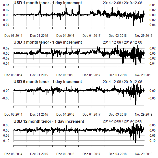
Stationarity in time series by 1-day differencing
We see that the upward trend from the interest rate time-series has gone, but from the period of April 2019 to November 2019 we see a lot of variation in the errors still the mean seems to be at zero. However, we could not be sure by just visualizing, we would run the Augmented Dickey-Fuller (ADF) test to be confident that the differenced time series is stationary.
library(tseries)
library(ggplot2)adf\_values = c()
for (i in 1:ncol(liborusd)){
  x = adf.test(liborusd\[,i\])
  adf\_values\[i\] = x$p.value}

#defining an increment dataframe
day1\_incu <- na.omit(diff(liborusd, lag = 1))
adf\_values\_1 = c()
for (i in 1:ncol(day1\_incu)){
  x = adf.test(day1\_incu\[,i\])
  adf\_values\_1\[i\] = x$p.value}
adf\_df <- data.frame(x = names(liborusd), val = adf\_values)
adf\_df\['inc\_1'\] = adf\_values\_1molten\_acf <- melt(adf\_df)
windows()
qplot(x,value, data = molten\_acf, color = variable, size = I(3)) +
  xlab ("LIBOR tenors for USD") + ylab ("Corresponding p-value in ADF") +
  ggtitle ("ADF test for stationarity")
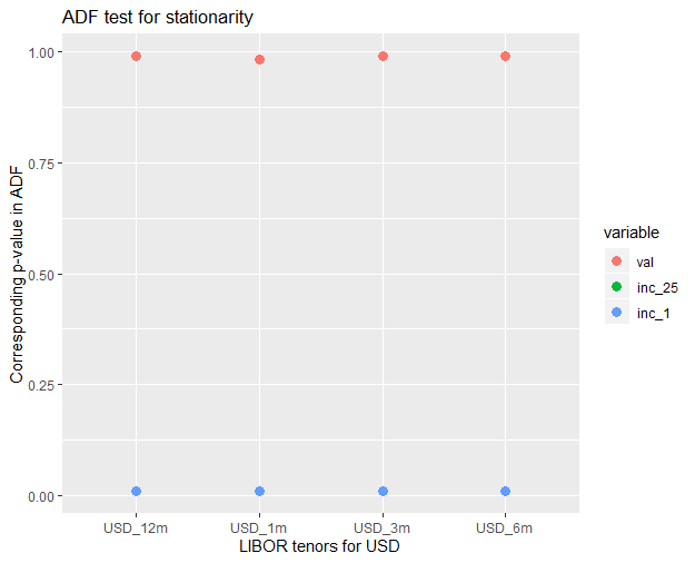
ADF test for stationarity of time series
So the ADF test, tests the null hypothesis that a unit root is present. The presence of unit root fails to reject non-stationarity of the series. At difference 1 in interest rate we could reject the null hypothesis. With a stationary time series we could now move ahead with fitting distributions.
Fitting Distributions to the Interest Rates Time Series
The differenced data represents the error of the time-series. This error is a stochastic contribution.For simplicity these distributions are considered symmetric with zero mean, a typical Gaussian shock, and is assumed to be product of volatility and noise. Let us plot the histogram to visualize the differenced data
#Slide 6 Plot IRs tenors with 1-day increment
windows(7,7)
par(mfrow=c(4,1))
plot(diff(liborusd$USD\_1m, lag =1, differences = 1),
     main = "USD 1 month tenor - 1 day increment")
plot(diff(liborusd$USD\_3m, lag =1, differences = 1),
     main = "USD 3 month tenor - 1 day increment")
plot(diff(liborusd$USD\_6m, lag =1, differences = 1),
     main = "USD 6 month tenor - 1 day increment")
plot(diff(liborusd$USD\_12m, lag =1, differences = 1),
     main = "USD 12 month tenor - 1 day increment")

Distribution of 1 day increment is similar to Gaussian distribution
It is clear from the graphs above that the tenors show normal like distribution. We could use the Cullen-Frey graph to compare distribution in skewness-kurtosis space. It gives the good summary of the distribution properties which we could use fitdistplus package in R.
library(fitdistrplus)
#Fitting one day increment distribution
descdist(as.numeric(day1\_incu\[,2\]), boot = 1000)#Fitting distribution
fn = fitdist(as.vector(day1\_incu$USD\_3m), "norm")
par(mfrow = c(2, 2))
plot.legend <- c("normal")
denscomp(list(fn), legendtext = plot.legend)
qqcomp(list(fn), legendtext = plot.legend)
cdfcomp(list(fn), legendtext = plot.legend)
ppcomp(list(fn), legendtext = plot.legend)
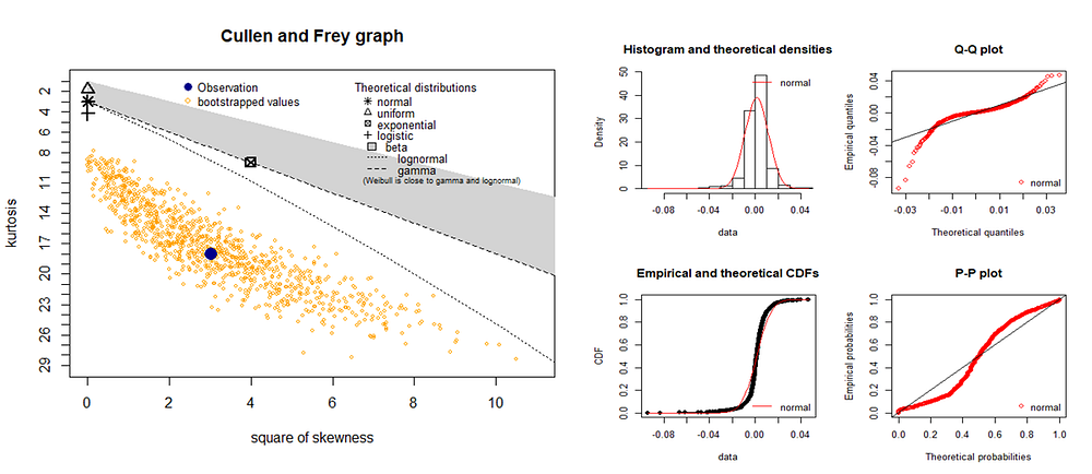
Cullen and Frey graph and fitting normal distribution
Now important part to understand here is that apart from getting pretty graphs what does this mean? In less words the answer to this is estimating the likelihood of the actual distribution with the theoretical distributions. And why do we do it? To help us find the appropriate distribution whose properties we know and whose behavior we could predict. So how is it done? By maximizing the likelihood function through fitting distribution we can rate the quality of statistical model by comparing AIC, BIC and log-likelihood (read more).
Simulating Vasicek/OU model
In the short rate modeling Vasicek model is a mathematical model which describes the evolution of interest rates. In its application in physical sciences it is also known as Ornstein-Uhlenbeck(OU) model. The model specifies that the instantaneous interest rate follows the stochastic differential equation:
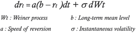
The above equation could help us solve the instantaneous volatility, speed of reversion and long-term mean level. The ‘sde’ package in R is a powerful package.
#Vasicek Model
\# The package defines a,b and sigma as theta\[2\],(theta\[1\]/theta\[2\]) and theta\[3\] respectively.
#Defining the expectation and variation of the modeldcOU <- function(x, t, x0 , theta , log = FALSE ){
  Ex <- theta \[1\] / theta \[2\]+( x0 - theta \[1\] / theta \[2\]) \* exp (- theta \[2\] \*t)
  Vx <- theta \[3\]^2 \*(1- exp (-2\* theta \[2\] \*t))/(2\* theta \[2\])
  dnorm (x, mean =Ex , sd = sqrt (Vx), log = log )
}
\# Defining a function for OU likelihood
OU.lik <- function( theta1 , theta2 , theta3 ){
  n <- length (X)
  dt <- deltat (X)
  -sum ( dcOU (X \[2: n\], dt , X \[1:(n -1)\] , c( theta1 , theta2 , theta3 ), log = TRUE ))
}
\# taking one tenor for the vasicek model fitting
X <- as.numeric(day1\_incu\[,1\])
mle(OU.lik, start = list( theta1 =0.01,
                          theta2 =2 ,
                          theta3 =0.05),
    method ="L-BFGS-B", lower =c(-Inf ,-Inf ,0.000001)) -> fit\# getting the model summary
summary(fit)
\# c**oef:** theta1 0.00246160, theta2 2.00126544, theta3   0.01381992#Plotting the simulation
y <- sde.sim( model ="OU", theta =unname(coef(fit)), N=1500, delta = 1)
plot(y, type="l", ylim=c(-0.04, 0.05), col = alpha(rgb(0,0,0), 0.1), main ="Simulation of Vasicek Model")
lines(ts(day1\_incu\[,1\]), col='red', type = "l")
The above line of codes would help us solve the equation. The important thing to note about this powerful package is that we specify the theta values but the package adjust the values on its own to maximize the likelihood.
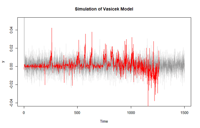
Vasicek Simulation for one of the interest rate tenor
By simulating the equations on the estimated parameters we would be able to average the variations and expectations to estimated the risk.
Conclusion
The aim of the article was to introduce the readers to time-series forecasting using SDE. We would have understood the basic rationale and a method to:
- Making time series stationary
- Fitting theoretical distributions
- Modeling on Vasicek/OU process
The readers are encouraged to engage and explore more about the statistical modeling. If the article has aroused more interest then it is encouraged to refer the book Option Pricing and Estimation of Financial Models in R by Stefano M Iacus on which the simulation of Vasicek Model is based.
Hope you would have enjoyed the reading leave your comments, thoughts and questions to further the discussion